Lec 27 Recap

Yesterday (Lec 27): We proved CLIQUE and Vertex Cover are NP-complete via reductions from 3-SAT.

• 3-SAT \le_P CLIQUE — clauses → groups of 3 vertices, edges across groups except conflicting literals
• CLIQUE \le_P Vertex Cover — complement graph duality: k-clique in G \iff (|V|-k)-vertex cover in \bar{G}

Consequence: Unless P = NP, no polynomial-time algorithm solves any of these optimally.

Coping with NP-Hardness

Three strategies when faced with an NP-hard problem:

Approximation Ratio

Example — Vertex Cover via Matching (Lec 26): Pick any edge, add both endpoints, remove incident edges, repeat.

|\text{Alg}| = 2 \cdot |M| \le 2 \cdot |\text{OPT}| \quad\Rightarrow\quad \text{2-approximation}

What is Linear Programming?

A linear program (LP) optimizes a linear objective subject to linear constraints.

Key fact: LPs can be solved in polynomial time (ellipsoid method, interior-point methods).

Geometric Intuition

LP Example: Product Mix

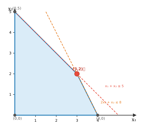
A factory produces two products P_1, P_2:

Available: 100 machine hours, 80 labor hours.

LP Formulation: \begin{aligned} \text{maximize} \quad & 40x_1 + 30x_2 \\ \text{subject to} \quad & 2x_1 + x_2 \le 100 \\ & x_1 + 2x_2 \le 80 \\ & x_1, x_2 \ge 0 \end{aligned}

Integer Programming

An Integer Program (IP) is an LP with integrality constraints:

\begin{aligned} \text{minimize} \quad & c^T x \\ \text{subject to} \quad & Ax \le b \\ & x \in \{0,1\}^n \quad (\text{or } \mathbb{Z}^n) \end{aligned}

Critical fact: IP is NP-hard. Adding integrality makes optimization exponentially harder.

Many NP-hard problems are naturally formulated as IPs.

LP Relaxation

Idea: Take an IP and “relax” the integrality constraints.

\begin{aligned} \text{IP:} \quad & \min c^T x, \; Ax \le b, \; x \in \{0,1\}^n \\ \text{LP Relaxation:} \quad & \min c^T x, \; Ax \le b, \; 0 \le x \le 1 \end{aligned}

Why this helps:

LP Rounding Framework

The general approach for LP-based approximation:

Example: Vertex Cover

Recall Vertex Cover: given graph G=(V,E), pick the minimum set of vertices touching every edge.

IP Formulation: \begin{aligned} \min \quad & \sum_{v \in V} x_v \\ \text{s.t.} \quad & x_u + x_v \ge 1 \quad \forall (u,v) \in E \\ & x_v \in \{0,1\} \end{aligned}

x_v = 1 means “vertex v is in the cover.” Constraint: for each edge, at least one endpoint is chosen.

Vertex Cover: LP Relaxation

Drop integrality — allow fractional values:

\begin{aligned} \min \quad & \sum_{v \in V} x_v \\ \text{s.t.} \quad & x_u + x_v \ge 1 \quad \forall (u,v) \in E \\ & 0 \le x_v \le 1 \end{aligned}

This is now a linear program — solvable in polynomial time.

Observation: The optimal LP value is a lower bound on the optimal IP value: OPT_{LP} \le OPT_{IP}

Because we’ve relaxed constraints — the feasible set is larger.

Vertex Cover: Rounding

We solve the LP and get fractional values x_v^* \in [0,1].

Rounding rule: Set \tilde{x}_v = 1 if x_v^* \ge \frac{1}{2}, else \tilde{x}_v = 0.

Feasibility: For any edge (u,v), x_u^* + x_v^* \ge 1. So at least one has x^* \ge \frac{1}{2}. Edge is covered. ✓

Approximation guarantee: |\tilde{x}| = \sum_v \tilde{x}_v \le 2 \sum_v x_v^* = 2 \cdot OPT_{LP} \le 2 \cdot OPT_{IP}

Thus we get a 2-approximation. ✓

Visualizing the Rounding

Edges with fractional cover values:

• Edge 1: x_u = 0.6, x_v = 0.4 → round u to 1
• Edge 2: x_u = 0.3, x_w = 0.7 → round w to 1
• Edge 3: x_v = 0.4, x_w = 0.7 → round w to 1

Each edge has at least one endpoint rounded to 1. Total covering cost ≤ 2 × fractional OPT.

When LP Rounding Works Best

LP rounding is a general recipe that applies to many NP-hard problems:

Key advantage: LP gives a principled lower bound on OPT — the hardest part of approximation analysis.

Summary

Next: More LP rounding applications — Set Cover, MAX-SAT, and randomized rounding.