BITS Pilani
CS F364: Design and Analysis of Algorithms

Models of Computation & Reductions

Lecture 26 |2026-07-10

Today’s Agenda

  1. Models of Computation
  2. Complexity Theory

How do computers work?

A vague answer

Silicon. Chips. Diodes. Logic gates. Transistors. Clock cycles. Machine instructions.

But do we need to know any of this to design algorithms?

Do we need all that?

No. We just need two things:

  1. Memory — to store data.
  2. A logical unit — to manipulate memory.

Algorithms came before computers

  • Euclid’s algorithm for GCD: ~300 BCE.
  • No silicon, no transistors — just a clear sequence of steps.

The same story is unfolding today

  • Quantum computers exist (experimentally).
  • But quantum algorithms (Shor’s, Grover’s) were designed years before working quantum hardware.
  • The algorithm came first — the machine followed.

The Turing Machine

Alan Turing (1936) gave us the simplest possible model of computation:
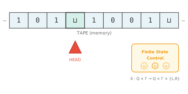
Components

  • An infinite tape divided into cells (memory).
  • A read/write head pointing to one cell.
  • A finite state control — a small set of states and rules.
  • A transition function \delta: given current state and symbol, decide what to write, which way to move, and what state to enter.

This is the formal definition of an algorithm. Everything you can do on any computer can be expressed as a Turing Machine.

The Church-Turing Thesis

Church-Turing Thesis

Any algorithm or computational process that can be performed by a physical machine or human can be simulated by a Turing Machine.

Other models, same power

  • RAM model, \lambda-calculus, counter machines, cellular automata…
  • All are polynomially equivalent — a problem solvable in O(f(n)) steps on one model is solvable in O(f(n)^c) steps on another.
  • This means we can analyze complexity without worrying about the specific machine.

Try the interactive Turing Machine from Google’s 100th birthday doodle — great way to see a TM in action.

Are all problems easy to solve?

No. There are inherently hard problems.

A Counting Argument (for fixed input length n)

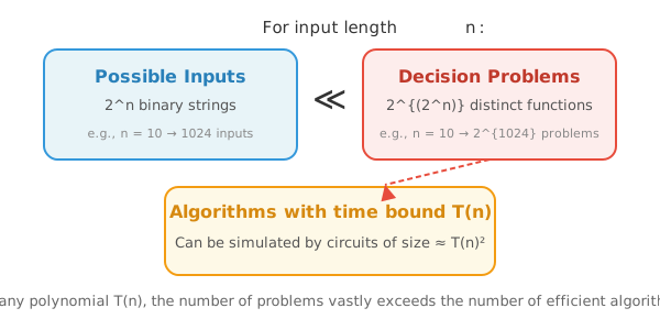
  • There are 2^n possible binary inputs of length n.
  • A decision problem maps each input to yes/no — that’s 2^{(2^n)} distinct problems.
  • An algorithm running in time T(n) can be simulated by a circuit of size \approx T(n)^2.
  • The number of distinct circuits of this size is far smaller than 2^{(2^n)}.

Therefore, most problems cannot be solved within any fixed polynomial time bound.
What this means

  • For any resource bound (time, memory), most problems exceed it.
  • Some problems are genuinely hard — not because we haven’t found a clever algorithm, but because none can exist within the bound.
  • Complexity theory is about classifying which problems are easy and which are hard.

Which are easy? Which are hard?

Complexity Theory is the study of this question:

  • Classify problems by the resources needed to solve them.
  • Time — how many steps does the algorithm take?
  • Space — how much memory does it use?
  • Group problems into complexity classes.

A preview

  • P: Problems solvable in polynomial time — “easy” (shortest path, sorting, MST).
  • NP: Problems verifiable in polynomial time — “easy to check” (Sudoku, Hamiltonian Cycle, SAT).
  • The big question: \text{P} \stackrel{?}{=} \text{NP}.

Decision Problems & Languages

To classify problems formally, we need a clean representation.

Encoding

Any problem instance (a graph, a matrix, a formula) can be encoded as a binary string in \Sigma^* = \{0, 1\}^*.

Decision vs Optimization

Instead of “Find the shortest path” (optimization), ask “Is there a path of length \le k?” (decision). Binary answer: yes or no. Maps directly to a formal language.

Formal Language

L \subseteq \Sigma^* = the set of all binary strings representing ‘yes’ instances.

Solving a problem = deciding membership: given x, is x \in L?

Comparing Difficulty: Reductions

Some problems feel harder than others. How do we prove it?

Karp Reduction (A \le_P B)

A polynomial-time function f such that:

x \in A \iff f(x) \in B
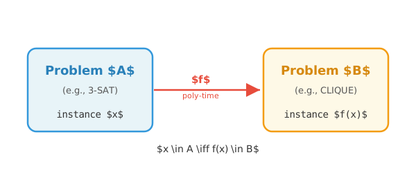
  • Transform any instance of A into an instance of B in polynomial time.

What this tells us

  • If B \in \text{P}, then A \in \text{P} (solve A by transforming to B).
  • Contrapositive: If A \notin \text{P}, then B \notin \text{P}.
  • Intuition: B is at least as hard as A.

The Hardest Problems: NP-Hardness

Reductions let us compare problems. What about the hardest problems?

Definition

A problem B is NP-hard if every problem in NP can be reduced to it:

\forall A \in \text{NP}: A \le_P B

If we could solve one NP-hard problem in polynomial time, we could solve every problem in NP — meaning \text{P} = \text{NP}.

What’s next?

In the next lecture, we will: 1. See concrete NP-complete problems — SAT, CLIQUE, Vertex Cover. 2. Work through explicit reductions step by step. 3. Understand the landscape of complexity classes.

The reduction idea you just learned is the key tool for all of this.