
CS F364: Design and Analysis of Algorithms
Randomized Algorithms
Lecture 25
|2026-07-10
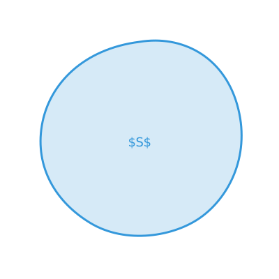
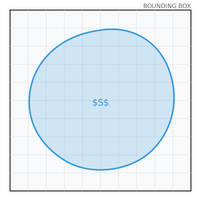
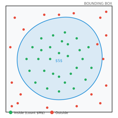
How do you compute the area of this shape?
Grid method: Superimpose a fine grid. Count cells that lie inside. Resolution-dependent and tedious.
A faster way — Random Sampling: 1. Enclose the shape in a bounding box. 2. Throw N darts uniformly at random. 3. Count M that land inside.
\text{Area}(S) \approx \text{Area}(\text{box}) \times \frac{M}{N}
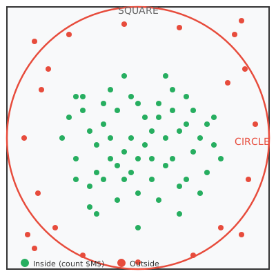
Circle of radius r inscribed in a square of side 2r:
\frac{\text{Area of circle}}{\text{Area of square}} = \frac{\pi r^2}{4r^2} = \frac{\pi}{4}
Throw N darts uniformly, M land inside:
\pi \approx 4 \cdot \frac{M}{N}
Randomized algorithms use random bits to guide their execution. They fall into two categories:
Problem: Given two polynomials P(x) and Q(x) of degree d, decide if they are identical (P(x) \equiv Q(x)).
Let P(x_1, \dots, x_n) be a non-zero polynomial of degree d over a field F. For a finite set S \subseteq F: \Pr_{r_1, \dots, r_n \sim S}[P(r_1, \dots, r_n) = 0] \le \frac{d}{|S|}
Given a bipartite graph G = (U, V, E), does it have a perfect matching?
Construct the Tutte matrix T where: T_{ij} = \begin{cases} x_{ij} & \text{if } (i,j) \in E \\ 0 & \text{otherwise} \end{cases}
Theorem (Lovász): \det(T) \not\equiv 0 \iff G has a perfect matching.
Evaluate \det(T) at random values (Schwartz-Zippel) → randomized matching test in O(n^\omega) time!
You wrote a program that computes something complex (e.g., determinant of a large matrix). How do you test if it’s correct for a given input?
Idea: Use the algebraic properties of the output. For a matrix multiplication program, check that A(Br) = Cr for a random vector r. A correct program will always pass; an incorrect one will fail with high probability.
This gives confidence in each individual run — far stronger than traditional testing.
Are two arithmetic expressions (e.g., (x-1)(x^4 + x^3 + x^2 + x + 1) and x^5 - 1) equivalent?
Instead of symbolically expanding both (exponential), pick random values and evaluate. Schwartz-Zippel guarantees: if they are different, the random test catches it with high probability.
This is used in computer algebra systems, compiler optimizations, and cryptographic protocol verification.
Problem: Alice and Bob have huge files (strings A and B) and want to check if they are identical (A = B) with minimal communication.
If A = B: always EQUAL.
If A \neq B: let x = A \oplus B \neq 0. Let i be the first bit where x_i = 1.
r \cdot x = r_1 x_1 + \dots + r_n x_n \pmod 2
For any fixed choice of r_1, \dots, r_{i-1}, r_{i+1}, \dots, r_n, exactly one value of r_i makes the sum 0. So:
\Pr[r \cdot x \equiv 0 \pmod 2] = \frac{1}{2}
Communication cost: n + 1 bits (the vector r plus one bit). Much better than transmitting the entire file!
Error: 1/2 per trial — we will fix this soon.
The idea of hashing/fingerprinting data to compare it cheaply appears everywhere:
Problem: Given three n \times n matrices A, B, C, verify that A \times B = C.
Deterministic: Multiply A \times B in O(n^\omega) time.
Randomized (Freivalds’): 1. Pick a random vector r \in \{0,1\}^n. 2. Compute A \cdot (B r) and C r in O(n^2) time each. 3. Output EQUAL if A(Br) = Cr, else DIFFERENT.
If C = AB: always EQUAL.
If C \neq AB: let D = AB - C \neq 0. Since D has at least one non-zero row, a random r \in \{0,1\}^n satisfies Dr \neq 0 with probability \ge 1/2.
Error: \le 1/2 per trial. Repeat k times → error \le 2^{-k}.
We have a Monte Carlo algorithm with error probability \delta per trial. How do we reduce it?
Run the algorithm k independent times (fresh randomness each time). Output “yes” only if all k trials say “yes”.
\Pr[\text{error after } k \text{ trials}] \le \delta^k
Suppose \delta = 1/2 and we run k = 30 trials:
\text{Error} \le \left(\frac{1}{2}\right)^{30} \approx 10^{-9}
This is far smaller than: * Probability of a hardware bit flip: \sim 10^{-10} per bit/hour * Probability of a cosmic ray strike: \sim 10^{-12} per gate * Probability of a data entry typo: \gg 10^{-6}
For all practical purposes, this is certainty.
Question for the Class
“If a Monte Carlo algorithm has error probability \delta = 1/3 per trial, how many independent trials do we need to match hardware error rates (\approx 10^{-12})?”
Answer: Solve (1/3)^k \le 10^{-12}.
k \ge \frac{12 \ln 10}{\ln 3} \approx \frac{12 \times 2.3026}{1.0986} \approx 25.1
So 26 trials suffice. The error drops from 0.333 to 10^{-12} — essentially zero.
We saw a recurring pattern throughout this lecture:
| Deterministic | Randomized | |
|---|---|---|
| Correctness | Always | With high probability (controllable) |
| Runtime | Often complex or slow | Simple and fast |
| Input dependence | Must handle worst case | Average case = worst case |
Randomized algorithms are simpler, faster, and more practical — the tiny controlled error is a bargain we take in practice.
Closing thought: As computer hardware continues to grow in scale, the probability of a hardware error in a long computation already exceeds the error we tolerate in a well-designed randomized algorithm. Randomization isn’t just a clever trick — it is often the more honest model of computation.
CS F364: Design & Analysis of AlgorithmsTulasimohan Molli