BITS Pilani
CS F364: Design and Analysis of Algorithms

Network Flow

Lecture 22 |2026-07-07
Today’s Agenda: Introduction to Network Flow

  1. Motivation & Applications
  2. Flow Network Definitions
  3. Capacity Constraints & Flow Conservation
  4. Residual Networks & Augmenting Paths

Recap: Lecture 21

Last lecture covered amortized analysis — proving sequences of operations have good average cost.

Today we start a new topic: Network Flow — a powerful framework for routing, matching, and scheduling.

1. Motivation: Flow Problems

We model transport networks where material moves from a source to a destination through capacity-constrained links.

Applications

  • Water/oil pipe networks
    • Graph = pipeline layout, vertices = junctions/reservoirs, edges = pipes, constraints = pipe diameters (max flow rate)
  • Data routing on the internet
    • Graph = network topology, vertices = routers/switches, edges = links, constraints = bandwidth limits
  • Transportation and logistics scheduling
    • Graph = transport network, vertices = hubs/depots, edges = routes, constraints = vehicle/road capacity limits <!– * Bipartite matching (next lecture)
    • Graph = worker-job assignments, vertices = workers + jobs, edges = possible assignments, constraints = each worker \le 1 job –>

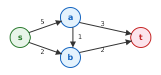
2. Flow Network: Visualized

Flow network

A flow network is a directed graph G = (V, E) with:

  • A source s and a sink t, each edge has capacity c(u,v) \ge 0.

3. Flow: Formal Definition

A flow is a function f: V \times V \to \mathbb{R} satisfying:

  1. Capacity Constraint: 0 \le f(u,v) \le c(u,v) for all u,v.
  1. Flow Conservation: For all v \neq s, t, \sum_{u} f(u,v) = \sum_{w} f(v,w) \quad\text{(inflow = outflow)}

Flow Value: |f| = \sum_{v} f(s,v) - \sum_{v} f(v,s), the net outflow from s.

4. Residual Networks

To find a maximum flow, we need to “undo” bad flow assignments.

Residual Capacity

For flow f, residual capacity of edge (u,v) is:

  • c_f(u,v) = c(u,v) - f(u,v) — room to push more forward
  • c_f(v,u) = f(u,v) — room to push back / undo flow

Residual Graph

G_f = (V, E_f) contains all edges with c_f(u,v) > 0.

5. Residual Graph: Visualized

After pushing flow f = 3 along s \to a \to t:
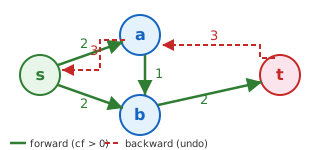
Residual graph

Forward edges (green): remaining capacity c_f = c - f Backward edges (red, dashed): capacity c_f = f to undo flow

6. Augmenting Paths

An augmenting path p is a simple path from s to t in the residual graph G_f.

Bottleneck Capacity

c_f(p) = \min \{ c_f(u,v) : (u,v) \in p \}

Augmentation Rule

Push c_f(p) along p:

  • Forward edges: f(u,v) \gets f(u,v) + c_f(p)
  • Backward edges: f(u,v) \gets f(u,v) - c_f(p)

7. Why Backward Edges Matter

Network: all edges capacity 1. Max flow = 2.

Flow network

Bad first choice: augment s \to a \to b \to t (flow = 1).

  • b \to t now saturated. Stuck with flow = 1. Not optimal.

8. Backward Edges Save Us

After s \to a \to b \to t (flow = 1):

  • Backward edges appear: b \to a (cap 1), t \to b (cap 1)
  • New augmenting path: s \to b \to a \to t
    • s \to b: forward (uses fresh capacity)
    • b \to a: backward (undoes a \to b)
    • a \to t: forward (redirects flow to sink)

Result: f(s,a) = 1, f(s,b) = 1, f(a,t) = 1, f(a,b) = 0, f(b,t) = 0. Total flow = 2 = maximum. ✓

9. Ford-Fulkerson: Preview

FORD-FULKERSON(G, s, t):
  for each edge (u,v): f(u,v) = 0
  while there exists an augmenting path p in G_f:
    cf(p) = min{cf(u,v) : (u,v) in p}
    augment f along p by cf(p)
  return f

Terminating Condition

Loop stops when no s \to t path exists in G_f — the residual graph has no augmenting paths.

Next lecture: Max-Flow Min-Cut Theorem proves this condition means the flow is maximum.

Concept Check: Network Flow

Question

“Why do we need backward edges in the residual graph?”

Answer: Backward edges allow us to redirect or ‘undo’ previous flow decisions that block us from the global maximum. Without them, a greedy choice can get stuck at a suboptimal flow.